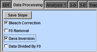
Bleach Correction
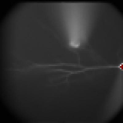
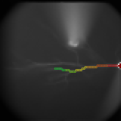
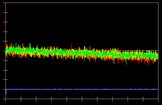
Five regions of interest (ROIs) were automatically selected along the apical dendrite (a). The automatic dendrite tracing procedure will be covered in tutorial #21. The imaging data in these ROIs are displayed in the imaging trace window (c). The color of each trace corresponds to the color of the respective ROI.
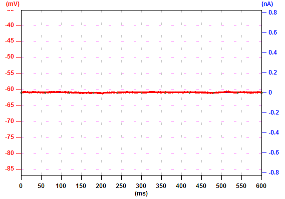
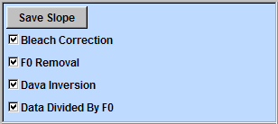
In the original data (c), you can see a deviation of the baseline. To correct this, click "Save Slope" button and check "Bleach Correction" (b). Now, the baseline deviation is corrected.
 (b)
(b) 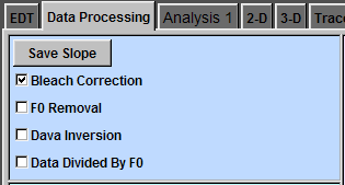
(c)
 (d)
(d) 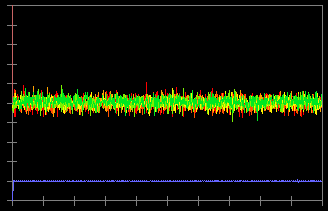
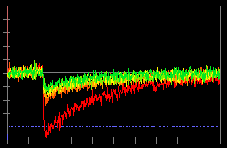
Data Inversion
In this record, an action potential was initiated from the soma by current injection (a). The neuron was filled with 100 µM bis-fura 2. The excitation wave length is 380 nm and the fluorescence light is collected from 470~550 nm. Due to this configuration, an increase in calcium concentration causes a decrease in fluorescence intensity (c). To inverse the data so an increase in calcium concentration corresponds to an increase in the trace, check "Data Inversion" (b) and the traces are inversed (d).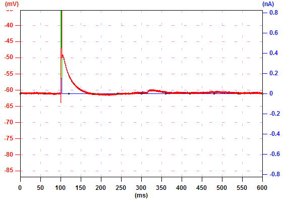
(b)
(c)
 (d)
(d) 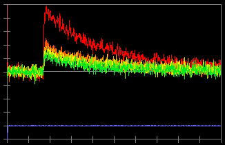
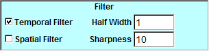
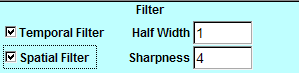
Temporal Filter
To reduce noise, you can use a digital temporal filter. Ephic provides a moving average filter. To specify the half width of the filter, type the number of points in "Half Window" box and press "Enter" (a). In this example, the half width is 1 point and Ephic will calculate the average from three points (2 x halfwidth + 1). By checking "Temporal Filter", the noise is reduced (b).
 (b)
(b) 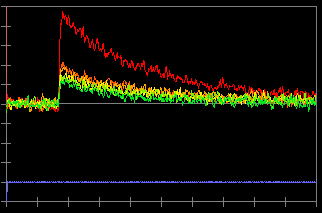
Spatial Filter
To reduce the noise in space, Ephic provides a 2-D filter. The kernal is a 3x3 matrix. You can control the sharpness of this filter by typing the sharpness index in "Sharpness" box and press "Enter". With larger index, you will have higher spatial resolution but larger noise in space. With lower index, you will have lower spatial resolution but lower noise in space.
In this example, the level of the original data is adjusted to show the spatial noise (b). To apply a spatial filter with a sharpness index of 4, type 4 in the "Sharpness" box and check "Spatial Filter". The spatial noise is lower now (c) but the spatial resolution is also lower.
(b)
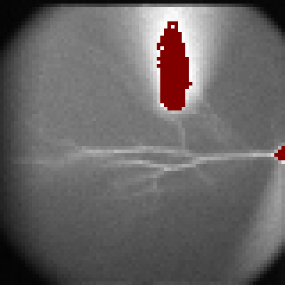 (c)
(c) 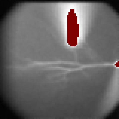
Calculate ΔF/F
To show ΔF/F in the imaging window, check "F0 Removal" box and "Data Divided by F0" box (a). To see the first frame, select "Snapshot" from the drop down menu. In this example, the signal amplitude of each pixel is seudocolored. The pixel between the centers of camera pixels is linearly interpolated.
 (b)
(b)
(c)
Movie
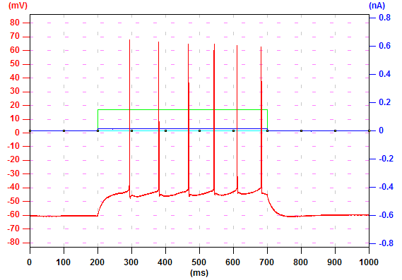
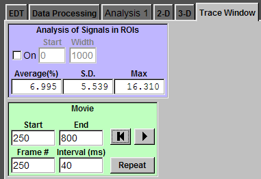
In this example record, six action potentials were evoked by current injection (a). To see the movie of back-propagating action potentials, click "Trace Window" tab (b). In "Movie" panel, enter the start point (250 pt), the end point (800 pt), and the interval between two frames (40 ms). The "Frame #" box displays the current frame number. Click play (the triangle button) and Ephic will display the movie. To pause the play, click play again. Panel (c) is the movie of calcium imaging signals evoked by these action potentials. You can ask Ephic to repeat the playback by check "Repeat". You can jump to the start frame by click the button with a bar and a triangle (b).
(b)
(c)
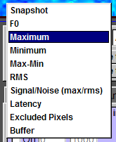
Maximum Amplitude Map
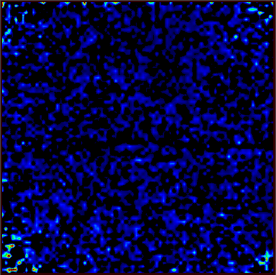
To display the maximum amplitude in the imaging window, select "Maximum" (a) and the imaging window will display the maximum amplitude map. From this map, you can see how far bAPs reach.
 (b)
(b) 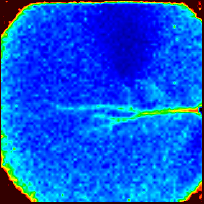
Pixel Exclusion
In some cases, you might want to exclude some pixels from analysis due to saturation of the pixels, low signal to noise ratio, or very noisy pixels. To do this, you need to set the period to calculate RMS values by entering the start and the width (pts) in the boxes by the label "Baseline (F0, RMS)" (b).
To mark saturated pixels and exclude them, click "Saturation" button and check the box next to it.
To set the S/N threshold, type the value in the box and press "Enter". To mark the mixels with S/N ratio lower the threshod and exclude them, click "Low S/N" button and check the box next to it.
To set the RMS threshold, type the value in the "RMS Threshold" box and press "Enter". To mark the mixels with RMS higher than the threshold, click "High RMS" button and check the box next to it.
By default, Ephic finds the maximum and other characteristics from the whole trace. If you want Ephic to find the maximum in a period (for example, to find the maximum amplitude in response to the second action potential), check the box next to "Analysis Window" (b) and enter the values (pts) in the boxes to specify the start and the width of this period.
 (b)
(b) 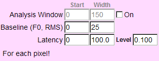
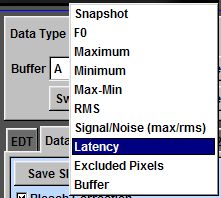
Latency
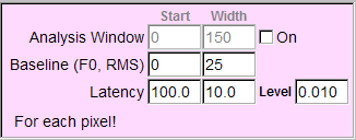
To display the latency of an event, set the threshold of the level in the box "Level". The pixel with the maximum amplitude lower than the level is considered as the background. Set the period to examine the latency. For example, to examine the events in the period from 100 to 110 ms, set values like panel (a). Ephic calculate the relative latency. For example, an event reaches the level of 0.01 at 100 ms is assigned an index of 1. An event reaches the level at 110 ms is assigned 0. An event reaches the level at 102 ms is assigned an index of 0.8. Thus, a larger index indicates a shorter latency.
To display the latency in the imaging window, click "Data Type" and select "Latency" (b).
 (b)
(b)